2. Constrained Dynamics

Curvilinear coordinates such as bond angles and Euler angles have coordinate singularities, where the transformation from Cartesian coordinates breaks down.

PySCIVR avoids this problem by propagating the dynamics in redundant coordinates with holonomic constraints (SHAKE/RATTLE), and transforms to the curvilinear coordinates only in the analysis, away from the singularities.

First, the pure rotation of H2 is used as an example:

Redundant space	Potential	Integrator	Physical space
Cartesian (6 DOFs) with 4 constraints (bond and 3 translations)	H2SplinePotential	ShakeRattle	2D sphere (polar \(\theta\) and azimuthal angle \(\phi\))

• The bond length and the center of mass are fixed by constraints.

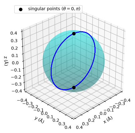
• The molecule rotates through the z-axis (\(\theta = 0, \pi\)), where the azimuthal angle \(\phi\) is undefined.

• H2SplinePotential is used as the potential.

• The trajectory is saved and loaded.

Note: For the pure rotation, the potential energy is constant, since it depends only on the shape of the molecule, which is fixed by the constraints. A constant potential affects neither the trajectory nor the monodromy matrix, so ZeroPotential gives the same results. Here, H2SplinePotential is used for consistency with the ro-vibration below.

# import necessary libraries

import numpy as np
import matplotlib.pyplot as plt
 
from pyscivr.coordinates import InternalCoordinates
from pyscivr.integrators import ShakeRattle
from pyscivr.potentials import H2SplinePotential
from pyscivr.save import load_trajectory, save_trajectory
from pyscivr.units import CmInv, FemtoSec

Set system

H2 is placed along the x-axis at the equilibrium bond length (\(r_e = 0.74160392 \AA\)).

mass = np.array([1.008, 1.008]) # mass of hydrogen atoms [amu (atomic mass unit)]
r_e = 0.74160392 # equilibrium bond length [Angs]
posi_ref = np.array([[-r_e / 2, 0.0, 0.0], [r_e / 2, 0.0, 0.0]])

calc = H2SplinePotential()
ener, force = calc.energy_forces(posi_ref)

print(f"Energy: {ener:.10f} eV")
print(f"Maximum force: {np.max(np.abs(force)):.10f} eV/Å")

Energy: -31.9530315756 eV
Maximum force: 0.0000001025 eV/Å

Set constraints

H2 has 6 Cartesian DOFs. We fix the center of mass (3 constraints) and the bond length (1 constraint), leaving 2 rotational DOFs.

Coordinates are defined by InternalCoordinates in the following steps:

1. Create an InternalCoordinates object with the reference positions posi_ref and the masses.

2. Add coordinates by the add_* methods, e.g. add_translation() for the center of mass and add_bond(i, j) for the bond length between atoms i and j. Bond angles, dihedral angles, polar and azimuthal angles, and Euler angles can be added in the same way.

3. Call build() to finalize the coordinate system.

When used as constraints, each coordinate is fixed to its value at the reference positions posi_ref, i.e., the constraint is \(F(q) = Q(q) - Q(q_{\text{ref}}) = 0\).

Here, the bond length is fixed to the equilibrium bond length r_e, and the center of mass is fixed to that of posi_ref.

All coordinates in coord_const are treated as constraints by ShakeRattle.

See pyscivr.coordinates for the full list of coordinates.

coord_const = InternalCoordinates(posi_ref, mass) # Initialize internal coordinates
coord_const.add_translation()
coord_const.add_bond(0, 1)
coord_const.build()
print(coord_const) # Prints the internal coordinates and their reference values

Build complete: 4 coordinates
InternalCoordinates:
    0: translation_x   value_ref=0.000000
    1: translation_y   value_ref=0.000000
    2: translation_z   value_ref=0.000000
    3: bond(0, 1)      value_ref=0.741604

Set initial conditions

The trajectory starts from the reference positions posi_ref: the molecule lies along the x-axis at the equilibrium bond length r_e, with the center of mass at the origin.

Since the constraints are defined at posi_ref, the initial positions satisfy them exactly. (ShakeRattle raises an error if the initial positions do not satisfy the constraints.)

The atoms are given opposite momenta perpendicular to the bond, so that the total momentum is zero and the bond length does not change, i.e., the initial momenta are also consistent with the constraints.

The molecule then rotates rigidly with the rotational kinetic energy K_rot \(\text{cm}^{-1}\).

tilt is the angle of the rotation plane from the xy-plane: with tilt = 0, the molecule rotates in the xy-plane and never passes through the z-axis, while with tilt = pi / 2, it rotates in the xz-plane and passes through the z-axis (\(\theta = 0, \pi\)) twice per rotation.

def initial_momenta(K_rot, K_vib, tilt):
    """Momenta for rigid rotation with the rotational kinetic energy K_rot [cm^-1] and vibrational kinetic energy K_vib [cm^-1]."""
    p_rot = np.sqrt(K_rot * CmInv * mass[0])
    p_vib = np.sqrt(K_vib * CmInv * mass[0])
    p_rot_y = p_rot * np.cos(tilt)
    p_rot_z = p_rot * np.sin(tilt)
    return np.array([[-p_vib, -p_rot_y, -p_rot_z], [p_vib, p_rot_y, p_rot_z]])
 
mome_init = initial_momenta(K_rot=2000, K_vib=0, tilt=np.pi/2)

Running the dynamics

The dynamics is propagated by ShakeRattle, which takes the potential, the initial positions and momenta, the masses, the time step, and the constraints coord_const.

• The time step must be given in the internal time unit; here it is converted from fs by multiplying FemtoSec.

• run(n_step) returns the trajectory as a dictionary of arrays. The initial state is included, so each array has n_step + 1 steps.

• In addition to the positions, momenta, forces and energies, the trajectory contains the Lagrange multipliers lam and mu of the constraints, which are needed for the propagation of the variations in the later tutorial.

The convergence of SHAKE can be controlled by the keyword arguments max_iter_shake and tol_shake (see the API reference).

dt_fs = 0.1 # time step in femtoseconds 
n_step = 5000

dt = dt_fs * FemtoSec # time step in internal units (Angs * sqrt(amu / eV))
 
dyn = ShakeRattle(calc, posi_ref, mome_init, mass, dt, coord_const)
traj = dyn.run(n_step)
t_fs = dt_fs * np.arange(n_step + 1)

print(traj.keys())

dict_keys(['posi', 'mome', 'potential_energy', 'force', 'total_energy', 'lam', 'mu', 'n_iter_shake', 'err_shake', 'dt', 'mass'])

Check energy conservation and constraint error

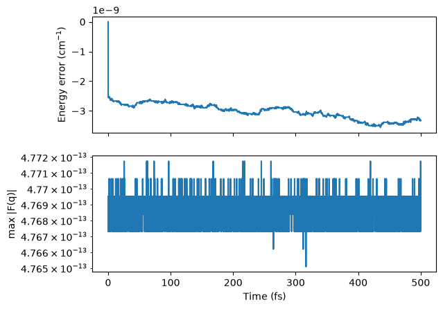
The total energy is conserved, and the constraints are satisfied within the SHAKE tolerance at every step.

ener = traj["total_energy"]
 
fig, axes = plt.subplots(2, 1, sharex=True)
axes[0].plot(t_fs, (ener - ener[0]) / CmInv)
axes[0].set_ylabel("Energy error (cm$^{-1}$)")
axes[1].semilogy(t_fs[1:], traj["err_shake"][1:])
axes[1].set_ylabel("max |F(q)|")
axes[1].set_xlabel("Time (fs)")
plt.show()

Save and load

If calculating trajectories is computationally expensive, they should be saved for reuse.

save_trajectory saves the positions, momenta, forces and energies.

The Lagrange multipliers lam and mu are not saved to reduce the file size, but can be restored from the trajectory by passing coord_const to load_trajectory.

The same constraints as used in the dynamics must be given; otherwise, the restoration fails with an error.

See pyscivr.save for details.

save_trajectory("h2_rot_pi2_traj.npz", traj)
traj_loaded = load_trajectory("h2_rot_pi2_traj.npz", coord_const=coord_const)

# Check if the saved and loaded trajectories are consistent
print("max |lam - lam_restored| =", np.max(np.abs(traj["lam"] - traj_loaded["lam"])))
print("max |mu - mu_restored|   =", np.max(np.abs(traj["mu"] - traj_loaded["mu"])))

max |lam - lam_restored| = 1.2248882463872235e-14
max |mu - mu_restored|   = 1.2241509889099333e-14

Visualize the trajectory in the Cartesian coordinate

posi = traj_loaded["posi"]                                 # (T, N, 3)
radius = r_e / 2                                           # distance of each atom from the center of mass

U = np.linspace(0, 2 * np.pi, 100)
V = np.linspace(0, np.pi, 100)
X = radius * np.outer(np.cos(U), np.sin(V))
Y = radius * np.outer(np.sin(U), np.sin(V))
Z = radius * np.outer(np.ones(np.size(U)), np.cos(V))

fig = plt.figure(figsize=(5, 5))
ax = fig.add_subplot(projection='3d', computed_zorder=False)

ax.plot_surface(X, Y, Z, color='cyan', alpha=0.3, zorder=0)
ax.plot(posi[:, 0, 0], posi[:, 0, 1], posi[:, 0, 2], color='blue', zorder=1)
ax.scatter([0, 0], [0, 0], [radius, -radius], color='black', s=50, depthshade=False,
           label=r'singular points ($\theta = 0, \pi$)', zorder=2)
ax.set_xlabel("x (Å)")
ax.set_ylabel("y (Å)")
ax.set_zlabel("z (Å)")
ax.view_init(elev=30, azim=45)
ax.set_box_aspect((1, 1, 1))
ax.legend(loc="upper left")
plt.show()

Convert to curvilinear coordinates

To analyze the rotation, we define a full set of 6 coordinates: the center of mass (3), the polar and azimuthal angles of the bond (2), and the bond length (1).

The number of coordinates equals the number of Cartesian degrees of freedom (\(3N = 6\)), so that the transformation between the Cartesian and curvilinear coordinates can be inverted.

The row order is changed by build(), so the row indices are obtained by find_coordinate.

The coordinate values are obtained by get_value(x) for a single geometry, or by get_value_batch(x) for a batch, where x is the flattened positions of shape (3N,) or (T, 3N). The lengths are in Å and the angles are in radians.

coord_all = InternalCoordinates(posi_ref, mass)
coord_all.add_translation()
coord_all.add_polar(0, 1)
coord_all.add_azimuthal(0, 1)
coord_all.add_bond(0, 1)
coord_all.build()
print(coord_all)
 
idx_polar = coord_all.find_coordinate("polar", (0, 1))[0]  # -> 4
idx_azim = coord_all.find_coordinate("azimuthal", (0, 1))[0]  #  -> 5
 
x = traj_loaded["posi"].reshape(n_step + 1, -1)  # (T, 3N)
values = np.asarray(coord_all.get_value_batch(x))  # (T, 6)
 
plt.plot(t_fs, values[:, idx_polar], label="polar")
plt.plot(t_fs, np.mod(values[:, idx_azim], 2 * np.pi), label="azimuthal")
plt.xlabel("Time (fs)")
plt.ylabel("Angle (rad)")
plt.legend()
plt.show()

Build complete: 6 coordinates
InternalCoordinates:
    0: translation_x   value_ref=0.000000
    1: translation_y   value_ref=0.000000
    2: translation_z   value_ref=0.000000
    3: bond(0, 1)      value_ref=0.741604
    4: polar(0, 1)     value_ref=1.570796
    5: azimuthal(0, 1) value_ref=0.000000

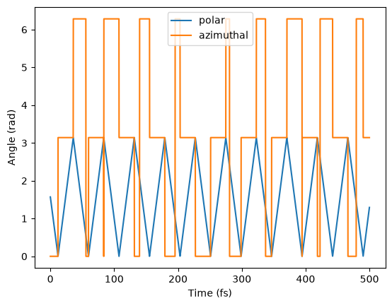
We can see that the azimuthal angle \(\phi\) jumps by \(\pi\) when the molecule crosses the z-axis (\(\theta = 0, \pi\)).

Exactly on the z-axis, \(\phi\) is undefined, since every value of \(\phi\) describes the same orientation (coordinate singularities).

The transformation from the Cartesian coordinates to \((\theta, \phi)\) therefore does not exist at these points, and its derivatives diverge in their vicinity, as shown below.

How to detect singularities

Whether the curvilinear coordinates \(Q\) are well defined at a geometry \(x\) can be checked by the gradient \(B = \frac{\partial Q}{\partial x}\), which is a \(3N \times 3N\) matrix for a full set of coordinates. The transformation can be inverted locally if and only if \(B\) is nonsingular.

A simple way to identify coordinate singularities is to monitor the condition number of \(B\), i.e., the ratio of its largest to smallest singular values, along the trajectory. The condition number diverges at a singularity, for either of two reasons:

• the smallest singular value goes to zero, i.e., the coordinates become linearly dependent, or

• the largest singular value diverges, i.e., the gradient of some coordinate diverges.

For the polar and azimuthal angles, the latter happens: the gradient of \(\phi\) is proportional to \(1 / \sin\theta\) and diverges on the z-axis.

On the other hand, the gradient \(B_C\) of the constraints used in ShakeRattle (center of mass and bond length) has no singularity along the trajectory, so the dynamics itself is not affected.

B_all = np.asarray(coord_all.get_const_grad_batch(x))     # (T, 6, 6)
B_const = np.asarray(coord_const.get_const_grad_batch(x))  # (T, 4, 6)
 
fig, axes = plt.subplots(2, 1, sharex=True)
axes[0].plot(t_fs, values[:, idx_polar])
axes[0].set_ylabel("Polar angle (rad)")
axes[1].semilogy(t_fs, np.linalg.cond(B_all), label="B (curvilinear coordinates)")
axes[1].semilogy(t_fs, np.linalg.cond(B_const), label="B_C (constraints)")
axes[1].set_ylabel("Condition number")
axes[1].set_xlabel("Time (fs)")
axes[1].legend()
plt.show()

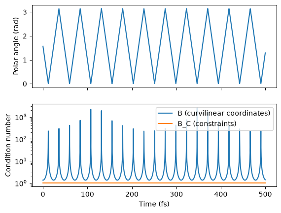
The condition number of B diverges whenever the polar angle \(\theta\) approaches \(0\) or \(\pi\), while that of B_C stays constant. Therefore, quantities that require the inverse of B should not be evaluated near these points e.g., the Hessian in the active coordinates by eval_hess_active (see the next tutorial).

Compare with a trajectory not passing the singularities

With tilt = pi / 4, the rotation plane is tilted by 45° from the xy-plane, so the polar angle stays between \(\pi / 4\) and \(3 \pi / 4\) and the trajectory never passes through the poles. The same coord_const and coord_all are used.

mome_init_pi4 = initial_momenta(K_rot=2000, K_vib=0, tilt=np.pi / 4)
traj_pi4 = ShakeRattle(calc, posi_ref, mome_init_pi4, mass, dt, coord_const).run(n_step)

ener_pi4 = traj_pi4["total_energy"]
print(f"max energy error = {np.max(np.abs(ener_pi4 - ener_pi4[0])) / CmInv:.3e} cm^-1")

x_pi4 = traj_pi4["posi"].reshape(n_step + 1, -1)                 # (T, 3N)
values_pi4 = np.asarray(coord_all.get_value_batch(x_pi4))        # (T, 6)
B_all_pi4 = np.asarray(coord_all.get_const_grad_batch(x_pi4))    # (T, 6, 6)

radius = r_e / 2
U = np.linspace(0, 2 * np.pi, 100)
V = np.linspace(0, np.pi, 100)

fig = plt.figure(figsize=(5, 5))
ax = fig.add_subplot(projection='3d', computed_zorder=False)
ax.plot_surface(radius * np.outer(np.cos(U), np.sin(V)), radius * np.outer(np.sin(U), np.sin(V)),
                radius * np.outer(np.ones(np.size(U)), np.cos(V)), color='cyan', alpha=0.3, zorder=0)
ax.plot(*traj_loaded["posi"][:, 0].T, color='blue', label=r'tilt = $\pi/2$', zorder=1)
ax.plot(*traj_pi4["posi"][:, 0].T, color='green', label=r'tilt = $\pi/4$', zorder=1)
ax.scatter([0, 0], [0, 0], [radius, -radius], color='black', s=50, depthshade=False,
           label=r'singular points ($\theta = 0, \pi$)', zorder=2)
ax.set_xlabel("x (Å)")
ax.set_ylabel("y (Å)")
ax.set_zlabel("z (Å)")
ax.set_box_aspect((1, 1, 1))
ax.view_init(elev=30, azim=45)
ax.legend(loc="upper left")
plt.show()

fig, axes = plt.subplots(2, 1, sharex=True)
axes[0].plot(t_fs, values[:, idx_polar], color='blue', label=r'tilt = $\pi/2$')
axes[0].plot(t_fs, values_pi4[:, idx_polar], color='green', label=r'tilt = $\pi/4$')
axes[0].set_ylabel("Polar angle (rad)")
axes[0].legend()
axes[1].semilogy(t_fs, np.linalg.cond(B_all), color='blue')
axes[1].semilogy(t_fs, np.linalg.cond(B_all_pi4), color='green')
axes[1].set_ylabel("Condition number of B")
axes[1].set_xlabel("Time (fs)")
plt.show()

max energy error = 2.608e-09 cm^-1

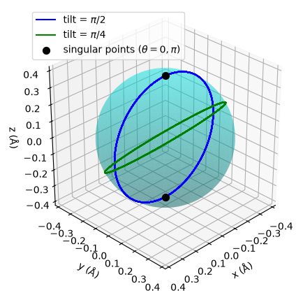
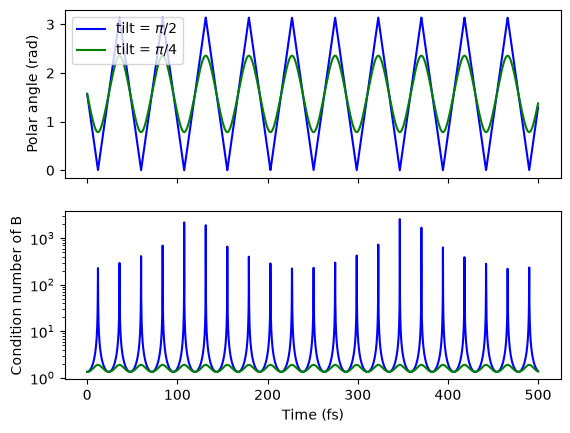
For tilt = pi / 4, the polar angle stays away from \(0\) and \(\pi\), and the condition number of \(B\) remains bounded.

The two trajectories have the same rotational energy and are physically equivalent: one is obtained from the other by rotating the whole system by \(\pi / 4\) about the x-axis. Nevertheless, only the trajectory with tilt = pi / 2 passes through the singular points. This shows that the coordinate singularity is not a physical property of the motion, but an artifact of the choice of the curvilinear coordinates (here, the direction of the z-axis). The dynamics in the redundant Cartesian coordinates is free from this artifact, and both trajectories are propagated equally well.

Second, the ro-vibration of H2 is used as an example:

Redundant space	Potential	Integrator	Physical space
Cartesian (6 DOFs) with 3 constraints (3 translations)	H2SplinePotential	ShakeRattle	bond length \(r\), polar \(\theta\) and azimuthal angle \(\phi\)

• The center of mass is fixed by constraints.

• The molecule rotates through the z-axis (\(\theta = 0, \pi\)), where the azimuthal angle \(\phi\) is undefined.

• The bond length is not constrained, so the molecule vibrates while rotating.

# Set constraints
coord_const_rovib = InternalCoordinates(posi_ref, mass)
coord_const_rovib.add_translation()
coord_const_rovib.build()
print(coord_const_rovib)

# set initial momenta
mome_init_rovib = initial_momenta(K_rot=2000, K_vib=2000, tilt=np.pi / 2)
traj_rovib = ShakeRattle(calc, posi_ref, mome_init_rovib, mass, dt, coord_const_rovib).run(n_step)

# check energy conservation
ener_rovib = traj_rovib["total_energy"]
print(f"max energy error = {np.max(np.abs(ener_rovib - ener_rovib[0])) / CmInv:.3e} cm^-1")

# save trajectory
save_trajectory("h2_rovib_pi2_traj.npz", traj_rovib)

# analyze trajectory
x_rovib = traj_rovib["posi"].reshape(n_step + 1, -1)                 # (T, 3N)
values_rovib = np.asarray(coord_all.get_value_batch(x_rovib))        # (T, 6)
B_all_rovib = np.asarray(coord_all.get_const_grad_batch(x_rovib))    # (T, 6, 6)


radius = r_e / 2
U = np.linspace(0, 2 * np.pi, 100)
V = np.linspace(0, np.pi, 100)

fig = plt.figure(figsize=(5, 5))
ax = fig.add_subplot(projection='3d', computed_zorder=False)
ax.plot_surface(radius * np.outer(np.cos(U), np.sin(V)), radius * np.outer(np.sin(U), np.sin(V)),
                radius * np.outer(np.ones(np.size(U)), np.cos(V)), color='cyan', alpha=0.3, zorder=0)
ax.plot(*traj_rovib["posi"][:, 0].T, color='blue', label=r'rovib (tilt = $\pi/2$)', zorder=1)
ax.scatter([0, 0], [0, 0], [radius, -radius], color='black', s=50, depthshade=False,
           label=r'singular points ($\theta = 0, \pi$)', zorder=2)
ax.set_xlabel("x (Å)")
ax.set_ylabel("y (Å)")
ax.set_zlabel("z (Å)")
ax.set_box_aspect((1, 1, 1))
ax.view_init(elev=30, azim=45)
ax.legend(loc="upper left")
plt.show()

bond_idx = coord_all.find_coordinate("bond", (0, 1))[0]  # -> 3

fig, axes = plt.subplots(3, 1, sharex=True, figsize=(6, 6))
axes[0].plot(t_fs, values_rovib[:, bond_idx], color='blue')
axes[0].set_ylabel("Bond length (Å)")
axes[1].plot(t_fs, values_rovib[:, idx_polar], color='blue')
axes[1].set_ylabel("Polar angle (rad)")
axes[2].semilogy(t_fs, np.linalg.cond(B_all_rovib), color='blue')
axes[2].set_ylabel("Condition number of B")
axes[2].set_xlabel("Time (fs)")
plt.tight_layout()
plt.show()

Build complete: 3 coordinates
InternalCoordinates:
    0: translation_x   value_ref=0.000000
    1: translation_y   value_ref=0.000000
    2: translation_z   value_ref=0.000000
max energy error = 4.062e+00 cm^-1

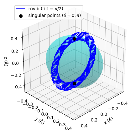
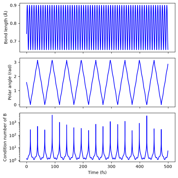
• Vibration: The bond length oscillates between about 0.65 Å and 0.90 Å with a period of about 8 fs, consistent with the vibrational frequency of H2 (about 4200 \(\text{cm}^{-1}\)). The oscillation is asymmetric around \(r_e\) (0.74 Å), reflecting the anharmonicity of the potential.

• Rotation: The polar angle shows small wiggles synchronized with the vibration. Since the angular momentum is conserved, the angular velocity decreases when the bond is stretched and increases when it is compressed. The rotational period (about 51 fs) is slightly longer than that of the pure rotation (about 48 fs), since the bond is longer on average.

• Singularities: The condition number of \(B\) diverges whenever the polar angle approaches \(0\) or \(\pi\), as in the pure rotation. The coordinate singularities depend only on the orientation of the molecule, not on the vibration.

• Trajectory on the sphere: The atoms move inward and outward from the sphere of radius \(r_e / 2\) while rotating through the poles. Since the vibrational and rotational periods are incommensurate, the trajectory does not close after one rotation.